In the last post, we started with f(x) = x3 + 4x and by some mysterious process, we generated a new formula, f’(x) = 3x2 + 4. This “derivative” tells us the slope of the original function’s tangent lines.
As you enter AP Physics, I would like you to be able to find the derivatives of some basic functions. I will let your math teachers explain where these formulas come from, but I want you to start getting familiar with these now.
Also, It is true that a TI-89 can find these derivative formulas for you. But the ones I am asking you to learn are so frequently encountered that it would be a waste of time to have to reach for a calculator. So let’s begin:
1. Constant Functions
Suppose f(x) = c, where c is a constant. The graph of f will be a horizontal line. The slope everywhere on that line is zero. So our first rule is an easy one:
If f(x) = c then f'(x) = 0
2. Linear Functions
Suppose f(x) = kx, where k is a constant. This graph will be a line passing through the origin with a slope, k. So this rule is also straight-forward:
If f(x) = kx then f'(x) = k
3. The Power Rule
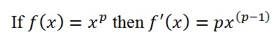
Some examples:
f(x) = x2 → f’(x) = 2x
f(x) = x3 → f’(x) = 3x2
f(x) = x4 → f’(x) = 4x3
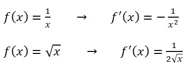
4. Power Rule, Special Cases
The power rule works for negative powers and for fractional powers. So you can use it to figure out the next two examples. But I think these two are worth memorizing so that you don’t have to stop to re-derive them…
5. Two Trig Functions
Your math teacher will teach you the derivatives of the functions for all six trigonometric ratios (and their inverse functions!) but for now, I’m just asking you to learn these two:
f(x) = sin(x) → f’(x) = cos(x)
f(x) = cos(x) → f’(x) = -sin(x)
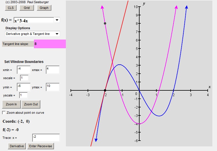
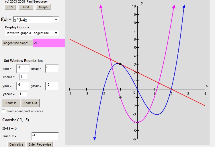
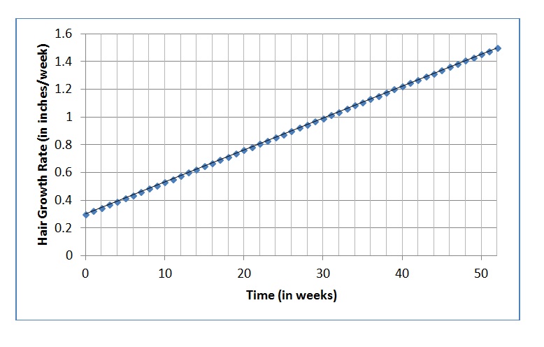
If you would like to be convinced that the derivative of the sine function is the cosine function, play the video.
Watch the tangent line surf along the sine wave (blue). Its slope changes in a pattern that matches the values of the cosine function (pink).
6. One more interesting function
There are many, many applications of exponential growth and decay in physics. Exponential functions are in the form:
![]()
where b is the base and x is the exponent.
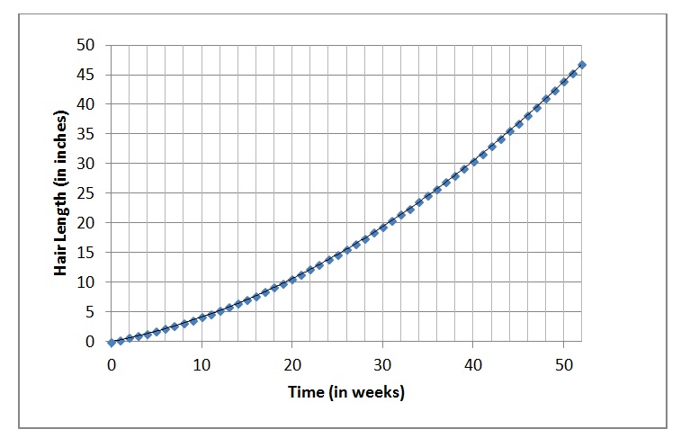
Here is the graph for the case when b = 2:

As long as the base is greater than one, exponential functions will all have this same characteristic shape.
There is, however, one special value for the base: the Euler number, e = 2.7182…
I sometimes think of e as π’s neglected cousin. They are both “transcendental” numbers, but I don’t know of any middle school that holds competitions for memorizing the digits of e. That may be because π is easier to explain: it’s the ratio of a circle’s circumference to its diameter.
But what is e? That’s a longer story (maybe for a future post — though there are entire books devoted to this subject). For now, I will tell you an interesting and important fact about e. The exponential function that has e as its base has a special property:
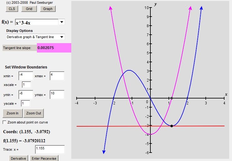
At every point along the graph of the function f(x) = ex, the slope of the tangent line at that point is equal to the value of the function at that same point.
Stop the movie at any point. Compare the value of the function to the slope of the tangent line until you can say “Aha!”
This gives us one more derivative rule:
![]()
Enough to Build on…
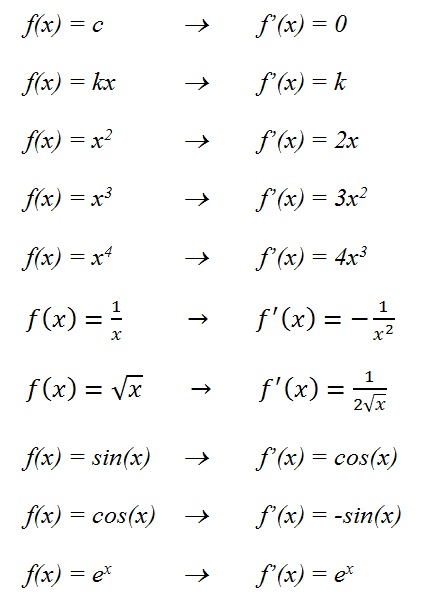
The basic rules you have seen in this post will get us through most of AP Physics. Now we have to learn how to apply these rules to combinations of functions. That’s coming next. For now, I’ll close by re-listing the rules. Memorize them. Print them out and put them in your notebook. Know them like you know your times-tables.