A Magical Theorem, Part II: Areas by way of Antiderivatives

So how are areas related to antiderivatives?  In other words (and symbols):

fundamentalquestion

This is the fundamental question.  When you know the answer, you will know the “Fundamental Theorem of Integral Calculus”.  But the main idea behind this all is something you have seen before in physics class (but not used quite this way).

In your first physics class, while studying kinematics, you learned that the area under a velocity vs time graph tells us the change in the object’s position.  To help jog your memory, play the video below:

The upper graph shows the velocity as a function of time for an object that happened to have a constant velocity of 10 m/s.

The lower graph shows the position vs time for the same object.  The velocity is constant so the position graph is linear with a constant slope.

On the velocity graph, you can see the area being swept out from t = 3 s to t = 7 s.  And on the position graph, you can see how far the object has moved during the same time interval.  Try stopping the animation at different times. Examine the graphs until you have convinced yourself of the following claim:

For a given time interval, the area under the Velocity vs. time graph will be equal to the change in position during that time interval.

YOU MAY BE SKEPTICAL…

After all, that was just with constant velocity.  But what if the velocity is changing?  Like so…

The velocity is increasing linearly and the position is increasing quadratically. [Remember, velocity is the derivative of position with respect to time. And the derivative of a 2nd-degree polynomial is a linear function.]

But even so, once again we see:

For a given time interval, the area under the Velocity vs. time graph will be equal to the change in position during that time interval.

STILL SKEPTICAL? STAY TUNED…

The velocity does not have to be changing linearly.  In fact, it does not even have to be velocity and position that we are talking about.  It can be any two quantities where one is the derivative of the other. Here’s one where the first graph is the rate at which water flows into a container and the second graph is the volume of water in that container:

Stop the animation at various points to check our claim:

If f(x) is the derivative of F(x), then the area under the graph of f(x) is equal to the change in F(x) over that same interval.

When we used this in 1st-year physics, we were using the area under the  DERIVATIVE (velocity vs time) to find the change in the original  function (position vs. time).  But now that we know how to find anti-derivatives, we can do this the other way around, using the change in the ANTI-DERIVATIVE (position) to find the area under the graph of the original function (velocity vs time).

And that answers the question we started with. What does area have to do with antiderivatives?  The area under the graph is equal to the change in the antiderivative.  That is called the Fundamental Theorem.  We write:

fundamentalanswer

WHY IS THIS USEFUL?

Well, suppose you want to find the area under some graph. This theorem gives you a procedure you can follow:

Step 1: Find an antiderivative.

Step 2. See how much the antiderivative changed by over the interval.

For example, suppose we want to know the area under the graph of f(x)=x2 between x=1 and x = 2, as illustrated below.

defintexample

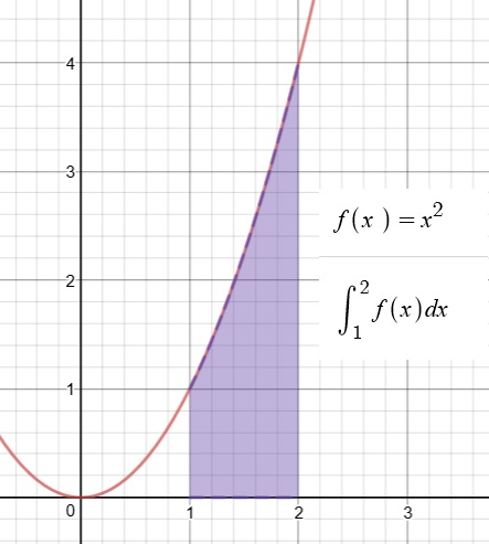
Let’s see.  Can we find an antiderivative?  Oh, yes, this one we did already.

F(x)=(1/3)x3 is an antiderivative of  f(x)=x2.

So now we just have to see how much F(x) has changed over the interval from x = 1 to x = 2.

F(3) = (1/3)(2)3 = 8/3

F(1) = (1/3)(1)3 = 1/3

F(3) – F(1) = 7/3

But what if I can’t find the antiderivative?

Well, that could be a problem.  That’s why you will spend so much time developing this skill in AP Calculus.  But I will reassure you again: in AP Physics, the antiderivatives you need will be manageable.  And there’s always Wolfram Alpha

Wait!  I don’t really understand how you can calculate the area of something with curvy boundaries. What does that even mean?

And I don’t understand: why does the area under the velocity graph equal the displacement?  Do we just have to accept that?

And I still don’t see why this is so important?  Are there lots of areas to be found in AP Physics?

These questions turn out to all be related!  See next post, Part III of our discussion of areas and integrals.


Ahead to Part III

Back to Part I

Go to Summer Reading Outline

A Magical Theorem: Antiderivatives and Areas, Part I

Sometimes in physics, we need to add up lots of little things.  In fact, an infinite number of infinitesimally small things.  When faced with this challenge, we use a method that takes advantage of a theorem so helpful and so concise that it feels like magic.

But the way we do this is really quite subtle.  You could master the method in math class and then still have trouble making the jump to using the method in physics class.  So in these next blog posts, I want to sort this out, even if just to help me organize my teaching.

Overview

Part I introduces the idea of an “anti-derivative” and it’s notation.  It also introduces a similar-and-yet-oh-so-different notation for area.  It turns out that when we talk about “integrating”, there are two different but related ideas that we might be referring to.  And we casually jump back and forth between them in a way that could easily blur the distinction.  So in this post, I try to at least make the distinction clear again.

Part II explains the connection between finding areas and finding anti-derivatives.  Essentially, this post introduces the Fundamental Theorem of Calculus (or Magic Theorem)  which gives us an easy way to find areas.  Part II closes by raising the question, “Why do we care so much about finding area in physics?”

Part III steps back and discusses Riemann Sums. This is the method we would have to use to find area if we did not have the Magic Theorem.  We won’t actually use this method, but we need to understand what the method does if we are going to understand “integrating” in physics.

Part IV revisits the question of finding displacement when velocity varies as a function of time.  So we will see one reason to find area (or integrate) in physics.

Part V (the last, I hope) will demonstrate how we use these area-finding methods whenever we need to add up a bunch of tiny little pieces.

OK, here we go…

Part I: “Integrals” — One word, Two meanings

If you have learned a little bit of calculus, even just by working your way through these Summer Reading posts, then at this point, you know how to find “derivatives” for a nice collection of reasonable functions.  Nothing too crazy or exotic — just the kinds of functions that you will meet early in AP Physics C.  And you also know why we find derivatives:  derivatives are slope-finding formulas.

For example:

Velocity is the rate of change of position with respect to time.

Acceleration is the rate of change of velocity with respect to time.

Force is the rate of change of momentum with respect to time.

Current is the rate of change of electric charge with respect to time.

For example, suppose you are given that an object moves so that it’s velocity as a function of time is:

v(t) = t2

You can easily find the acceleration as function of time by taking the derivative:

a(t) = v’(t) = 2t

So there are good, useful reasons for learning how to find derivatives. (In fact, let me remind you that to “optimize” a function, you usually begin by finding the derivative and then setting it equal to zero.)

CAN WE PLAY THE GAME IN REVERSE?

If I give you a function, can you find an “antiderivative”?

For example, let’s say:  f(x)=x2

Can we find another function that has f(x)=x2 as its derivative? If we know the basics, finding this particular antiderivative is not that hard:

F(x)=(1/3)x3

But you don’t have to take my word — go ahead an take the derivative!  You will see for yourself that the derivative of F(x)=(1/3)x3 is indeed f(x)=x2.

(But also, in this case you can see where we got this: taking a derivative lowers the power so we better raise the power by 1.  Oh, and the power will come out in front as a multiplier, so we stick in a factor of 1/3 to cancel that…)

So  F(x)=(1/3)x3 is an antiderivative of  f(x)=x2.

But it is not the only one!  Try taking the derivative of any of these:

F(x)=(1/3)x3 + 5

F(x)=(1/3)x3 – 99

F(x)=(1/3)x3 + C where C is a constant

So if you can find one antiderivative, you can find a whole family of them.  Still, most times, you only need to find one.

[Caution: your math teacher will likely take off a point or two if you leave out the “…+ c” when finding an antiderivative. They are kind of obsessive about this.  ]

IS IT ALWAYS THIS EASY?

Well, no.  Some antiderivatives are easy to find.  But others…not so much.  You will spend a substantial amount of time in math class building a collection methods for finding antiderivatives for an increasing variety of functions.  Some of these methods are quite subtle.  You can easily start to think that this quest for antiderivatives is what it means to do calculus.  But it is really just a means to a more useful end, not the main event.  And in fact, there are even functions that don’t have antiderivatives whose formulas we can find!

For now, I want to make two points:

1. In our AP Physics class, the antiderivatives we need will mostly be pretty easy to find.  You will be able to use “guess and check” to find them.  And if they ARE  hard to find, you can have a little help: your TI89s or N-Spires know how to do this.  So does Wolfram Alpha.

2. Nobody would be willing to invest so much effort in finding antiderivatives unless there was something really useful about them! We will get to that soon. But first:

A NEW NOTATION

If we are going to be using antiderivatives, we should have symbols for writing them.  To indicate that F(x) is the antiderivative of f(x), we write:

indefint1

This is just another way of saying that F'(x) =  f(x).  And, in addition to calling F(x)  an antiderivative, we also sometimes call it the “indefinite integral of f(x)”.

BUT WAIT…

On the other hand, there is another symbol that looks almost the same but means something completely different:

defint

This symbol is called the “definite integral” (as opposed to “indefinite”).  It is not a function at all! Just adding values at the top and bottom of that strange elongated s-shape gives the symbol a whole new meaning:

The definite integral is the area of the region bounded by the function, the x-axis and the two “limits of integration”: the vertical lines defined by x=a and x=b.

For example, here is a definite integral:

defint1

And here is the area that definite integral is referring to:

area1

So now we have two very different ideas that have been given very similar symbols and names. It would be easy to get these two things confused…

There is the INDEFINITE INTEGRAL:

indefint1

This is a FUNCTION which has f(x) as its derivative.

And then there is the DEFINITE INTEGRAL:

defint

This is an AREA — a numeric value.

And now the big question:

Why do mathematicians use these similar names and symbols for these two very different ideas?  Are they secretly related in some FUNDAMENTAL way?  

That is the topic of the next post, Part II of this discussion.

Ahead to Part II

Go to Summer Reading Outline