Sometimes in physics, we need to add up lots of little things.  In fact, an infinite number of infinitesimally small things.  When faced with this challenge, we use a method that takes advantage of a theorem so helpful and so concise that it feels like magic.

But the way we do this is really quite subtle.  You could master the method in math class and then still have trouble making the jump to using the method in physics class.  So in these next blog posts, I want to sort this out, even if just to help me organize my teaching.

Overview

Part I introduces the idea of an “anti-derivative” and it’s notation.  It also introduces a similar-and-yet-oh-so-different notation for area.  It turns out that when we talk about “integrating”, there are two different but related ideas that we might be referring to.  And we casually jump back and forth between them in a way that could easily blur the distinction.  So in this post, I try to at least make the distinction clear again.

Part II explains the connection between finding areas and finding anti-derivatives.  Essentially, this post introduces the Fundamental Theorem of Calculus (or Magic Theorem)  which gives us an easy way to find areas.  Part II closes by raising the question, “Why do we care so much about finding area in physics?”

Part III steps back and discusses Riemann Sums. This is the method we would have to use to find area if we did not have the Magic Theorem.  We won’t actually use this method, but we need to understand what the method does if we are going to understand “integrating” in physics.

Part IV revisits the question of finding displacement when velocity varies as a function of time.  So we will see one reason to find area (or integrate) in physics.

Part V (the last, I hope) will demonstrate how we use these area-finding methods whenever we need to add up a bunch of tiny little pieces.

OK, here we go…

Part I: “Integrals” — One word, Two meanings

If you have learned a little bit of calculus, even just by working your way through these Summer Reading posts, then at this point, you know how to find “derivatives” for a nice collection of reasonable functions.  Nothing too crazy or exotic — just the kinds of functions that you will meet early in AP Physics C.  And you also know why we find derivatives:  derivatives are slope-finding formulas.

For example:

Velocity is the rate of change of position with respect to time.

Acceleration is the rate of change of velocity with respect to time.

Force is the rate of change of momentum with respect to time.

Current is the rate of change of electric charge with respect to time.

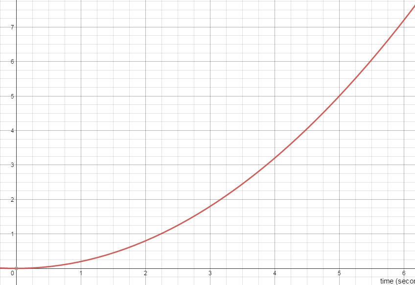
For example, suppose you are given that an object moves so that it’s velocity as a function of time is:

v(t) = t²

You can easily find the acceleration as function of time by taking the derivative:

a(t) = v’(t) = 2t

So there are good, useful reasons for learning how to find derivatives. (In fact, let me remind you that to “optimize” a function, you usually begin by finding the derivative and then setting it equal to zero.)

CAN WE PLAY THE GAME IN REVERSE?

If I give you a function, can you find an “antiderivative”?

For example, let’s say:  f(x)=x²

Can we find another function that has f(x)=x² as its derivative? If we know the basics, finding this particular antiderivative is not that hard:

F(x)=(1/3)x³

But you don’t have to take my word — go ahead an take the derivative!  You will see for yourself that the derivative of F(x)=(1/3)x³ is indeed f(x)=x².

(But also, in this case you can see where we got this: taking a derivative lowers the power so we better raise the power by 1.  Oh, and the power will come out in front as a multiplier, so we stick in a factor of 1/3 to cancel that…)

So  F(x)=(1/3)x³ is an antiderivative of  f(x)=x².

But it is not the only one!  Try taking the derivative of any of these:

F(x)=(1/3)x³ + 5

F(x)=(1/3)x³ – 99

F(x)=(1/3)x³ + C where C is a constant

So if you can find one antiderivative, you can find a whole family of them.  Still, most times, you only need to find one.

[Caution: your math teacher will likely take off a point or two if you leave out the “…+ c” when finding an antiderivative. They are kind of obsessive about this.  ]

IS IT ALWAYS THIS EASY?

Well, no.  Some antiderivatives are easy to find.  But others…not so much.  You will spend a substantial amount of time in math class building a collection methods for finding antiderivatives for an increasing variety of functions.  Some of these methods are quite subtle.  You can easily start to think that this quest for antiderivatives is what it means to do calculus.  But it is really just a means to a more useful end, not the main event.  And in fact, there are even functions that don’t have antiderivatives whose formulas we can find!

For now, I want to make two points:

1. In our AP Physics class, the antiderivatives we need will mostly be pretty easy to find.  You will be able to use “guess and check” to find them.  And if they ARE  hard to find, you can have a little help: your TI89s or N-Spires know how to do this.  So does Wolfram Alpha.

2. Nobody would be willing to invest so much effort in finding antiderivatives unless there was something really useful about them! We will get to that soon. But first:

A NEW NOTATION

If we are going to be using antiderivatives, we should have symbols for writing them.  To indicate that F(x) is the antiderivative of f(x), we write:

This is just another way of saying that F'(x) =  f(x).  And, in addition to calling F(x)  an antiderivative, we also sometimes call it the “indefinite integral of f(x)”.

BUT WAIT…

On the other hand, there is another symbol that looks almost the same but means something completely different:

This symbol is called the “definite integral” (as opposed to “indefinite”).  It is not a function at all! Just adding values at the top and bottom of that strange elongated s-shape gives the symbol a whole new meaning:

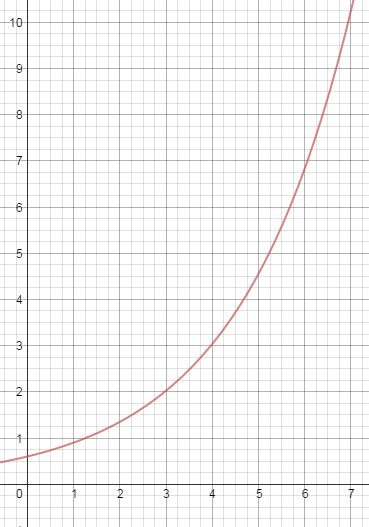
The definite integral is the area of the region bounded by the function, the x-axis and the two “limits of integration”: the vertical lines defined by x=a and x=b.

For example, here is a definite integral:

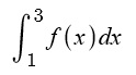
And here is the area that definite integral is referring to:

So now we have two very different ideas that have been given very similar symbols and names. It would be easy to get these two things confused…

There is the INDEFINITE INTEGRAL:

This is a FUNCTION which has f(x) as its derivative.

And then there is the DEFINITE INTEGRAL:

This is an AREA — a numeric value.

And now the big question:

Why do mathematicians use these similar names and symbols for these two very different ideas?  Are they secretly related in some FUNDAMENTAL way?  

That is the topic of the next post, Part II of this discussion.

Ahead to Part II

Go to Summer Reading Outline

“Is that the kind of thing you just have to memorize?”

That’s a question that should make a math teacher nervous.  There are certainly procedures and formulas that are occasionally useful to memorize.  But not “just” memorize!  If we don’t aim for a deeper understanding, then we have lost sight of why we are doing any of this.  In fact, if we never even try to have our students understand some particular piece of mathematics, then that piece is a good candidate to drop from the curriculum. (I’m looking at you, Descartes Rule of Signs).

On the other hand, we do want our students to be able to do a lot of things!  And the reasons behind some of them are sometimes more subtle or more advanced than what students need to hear at the moment they are first learning them.  So it can be a bit of a balancing act — finding the right degree of explanation and rigor at every level.

One somewhat disheartening thing I see at the high school level is that my students don’t seem to expect to understand the rules.  They have been graded on their ability to replicate a startling number of procedures.  That these things can be understood seems almost beside the point to them.  I wish we taught a whole lot more about a whole lot less…

So what has me started on this rant on a lovely snow day in the new year?  Well, while not grading a pile of papers, I came across a twitter discussion of this question:

Why is a negative times a negative a positive?

As you ponder this issue, you see that it is related to:

Why is a positive times a negative a negative?

I would like to offer an answer that requires no algebra — so it can be used with the students who are first learning these rules.

GUIDING IDEA

Often in math, we start with an idea that has one interpretation and then we extend it into new areas that cause us to expand or even give up the original interpretation. But we try to extend the idea in ways that continue the rules and patterns that we had before.

So for example, when you first learned to multiply, say 5 × 4 = ?

You can think of that as 5 sets of 4.  (Or 4 sets of 5!)

You can make rows of dots:

•    •    •    •

•    •    •    •

•    •    •    •

•    •    •    •

•    •    •    •

But now someone asks you to multiply a positive times a negative: 5 × -4 = ?

I don’t know how to make 5 rows with -4 dots in a row.  Or -4 rows with 5 dots in each.  So to answer this question, I am going to have to extend what it means to multiply.  But I want to keep patterns intact.  What kind of patterns? Well, here’s one:

5 × 4 = 20

5 × 3 = 15

5 × 2 = 10

5 × 1 = 5

5 × 0 = 0

Hmm.  When you are multiplying 5 by successively smaller whole numbers, your answer decreases by 5 each time.  What if we want that pattern to continue?

5 × -1 = -5

5 × -2 = -10

5 × -3 = -15

5 × -4 = -20  Aha!  That was the question we started with.  We just found a way to multiply a positive by a negative.

[If all you care about is getting the answer, then you memorize the procedure: to multiply a positive by a negative, just multiply the “regular” way and then make your answer negative.  But without some understanding, it feels so hollow.]

But wait!  There’s more…

Now someone asks you to multiply, say:  -4 × -5 = ?

I still don’t know how to draw -5 rows each with -4 dots.  But I can look for patterns!

We have learned how to multiply positives and negatives. So for example…

4 × -5 = -20

3 × -5 = -15

2 × -5 = -10

1 × -5 = -5

0 × -5 = 0

Any pattern?  Hmmm.  When you multiply -5 by successively decreasing whole numbers, the products INCREASE by 5 each time…and if we continue the pattern:

-1 × -5 = +5

-2 × -5 = +10

-3 × -5 = +15

-4 × -5 = +20  Aha (again)!  We have our answer — not because we “just” memorized that a negative times a negative is a positive, but because that is the way it has to be for our pattern to be extended.

The idea of developing new rules in a way that maintains old patterns will certainly be useful again. In fact, I just remembered another example of this.  I once gave a guest lesson to a 5th grade class that wanted to know why a number raised to the power of zero is 1.  I came up with a kind of lengthy explanation involving the laws of exponents…I don’t know how many hearts and minds I won that day.  Then I went home and thought about it a little more.  I came back the following day with a much shorter lesson:

2^5 = 32

2^4 = 16

2^3 = 8

2^2 = 4

2^1 = 2

What happens to the answer each time you lower the exponent by 1?  Keep that pattern going…

And keep it going further, to learn more than you expected!

Since I started this blog, one recurring goal has been to explore ways to visualize mathematical ideas.  In that spirit,  I spent a few posts talking about this diagram here:

These three posts discuss the development of this diagram:

Also Better With Pictures — The Trigonometry Ratios

Picturing the Trigonometric Ratios: Step-by-step

Trig Pictures, Part III

Whenever I show this diagram to students, they seem actually excited to discover the meaning and reasons behind so much trigonometry that they had previously just memorized.  It makes me believe that it would be helpful if this diagram was displayed in every room where trigonometry is introduced.  And now it can be!  I tidied up the graphics and made it into a poster.

Here it is, available to download, in two convenient sizes:

For your notebook (8.5″ x 11″)  Trig Diagram Notebook-sized

For your wall (22″ x 28″ ) Trig Diagram Poster-Sized

Also, I recently gave a workshop about this. You can see the slides here.

COMING SOON: T-SHIRTS!!  (Maybe)

UPDATE 11/1/2017 My obsession continues…now you can see an animated version.  I made this in Desmos.  You can see it here:

 https://www.desmos.com/calculator/mvj7yljovi

Now, how do I get THAT on a t-shirt?

The other day, a colleague showed me a diagram about current vs. time in an RC circuit. The diagram helped me realize that there is another way to think about time constants and exponential decay, a way I had completely overlooked.  I had all the right pieces floating around but I had never put them together. 

WHAT’S A TIME CONSTANT?

Here are three graphs showing a quantity that is decaying exponentially toward zero:

Each of these is a graph of a function: N(t) = N_oe^-kt

The only difference is the value of the constant, k.  Higher values of k lead, in a sense, to faster decay.

To help emphasize this, we can define a constant: τ = 1/k

Then we can  re-write the function this way: N(t) = N_oe^-t/τ

We call τ the “time constant” for this decay.  It has the units of time.  And it gives us an intuitive feeling for how fast a function is decaying.

For every time constant that passes, our decaying quantity gets reduced by another factor of e.

So after one time constant has passed, the function’s value is N_o/e.  After two time constants, it’s N_o/e².  After three, N_o/e³ …and so on.

But there is another way to think about the time constant.

The time constant tells us how long it would take to reach the asymptote at the current rate of change.

Maybe this should have been obvious, but I never thought about that way until just a few days ago. Here’s the diagram that got me started:

http://www.algebralab.org/practice/practice.aspx?file=Reading_ChargingCapacitor.xml

The claim here is made in the context of a charging capacitor, but it is actually true for any function that is approaching an asymptote exponentially. Here is an animation I made in Desmos to illustrate the point:

In the still picture above, you can see the tangent line at t=0.  The dotted green segment on the t-axis represents the time it would take for the tangent line to reach the asymptote.  When you run the video, you will see the function decrease and the tangent line get shallower.  But that green segment stays the same length.

(If you want to play with the Desmos file, you can get it here🙂

WAIT – WHAT’S A TIME CONSTANT NOW?

A quantity that decays exponentially approaches its final value asymptotically. And as it decays, its rate of decay decreases as well.  (That’s the defining characteristic of exponential decay: the rate of decay toward the final value is proportional to the current distance from that value.  In fact, we can write that as a differential equation. I went on and on about that here.)

But now suppose that at some moment, the decay rate were to become constant. Instead of taking forever, the function would now be able to reach its asymptote in a finite amount of time. Not in just any old amount of time, but in fact in an amount that equals the “time constant” of the decay. It doesn’t matter what moment you pick.  From any starting point during exponential decay, if the rate were to stay constant (which it doesn’t, but still…) the time to reach the asymptote would always comes out to τ = 1/k.

Or to say the same thing geometrically: the tangent line from any point on the curve will intercept the asymptote after one time constant has elapsed. That’s what the animation is trying to emphasize.  I chose a k value of .2 so my time constant was 1/.2 = 5 seconds.  If you open the Desmos file, you can change the constants to see what changes and what doesn’t.

SO WHY DID THIS SURPRISE ME?

I wasn’t making the connection between the exponential decay and the differential equation lurking in the background (even though I teach that connection and have blogged about it).

That the function decreases with a rate of change that is proportional to the value of the function is actually a first-order differential equation.  The exponential decay is its solution. (Again, gory detail here.)

And if slope is rise over run, then run is rise over slope!  When the function is starting from a higher value, the tangent has a slope that is PROPORTIONALLY higher!  So that proportionally higher slope will get you back to the asymptote in the same amount of time every time.

To find how much time we are talking about, divide the “rise” (or in this case, a “fall”) by the slope:

I’ll leave a more rigorous, math-y proof as an exercise for those of you in your first calculus class.

And now he asks:

“If I roll a die five times, how many distinct values should I expect to see?”

I was feeling pretty good about myself having solved the first one. (Here) And my Excel simulation told me I was at least close.  But when I attacked this new one, I hit some trouble.  I know I need the expected values, but to get them, I need the probabilities.  And I was bogging down in the calculations.  I could find the probability of getting one distinct value, but two was harder, three harder still…

Simulate first and calculate later

I already had the spreadsheet with the random integers.  But Excel does not have a “number of discrete values on the list” function.  So even there, I was stuck.

[Side note: back in the day when I did know how to code, I briefly knew an obscure programming language called APL.  I believe that in APL, a problem like this can be solved in a single line of code, dense with obscure symbols.  Document your code, campers, or you will never remember what you did!]

But since JT only rolled the dice 5 times, I did eventually come up with a way to have Excel do this for me. Let’s call it the “Go Fish” procedure, naming it after the simple card game.  It’s not very elegant but it works and, as you will see, it pays extra dividends.

For each possible dice value, 1 through 6, I made a column that answered the question: did this value appear on the list. For example, the formula in my first column answers the Go Fish question: got any ones?

=1×or((a2=1),(b2=1),(c2=1),(d2=1),(e2=1))

This generates a value of 1 if any of the dice came up as a 1 and zero if none of them did.

I made a total of 6 columns like this. Then, the sum of those columns tells me how many distinct values appeared in my original 5 rolls of the dice.

From there, it was just a matter of doing this in every row and taking the average. Again I did 10 years worth of rows.

You can see in the top row that the dice came up: 1, 3, 2, 1, 1

So the answer was yes if the question was got any 1’s, 2’s or 3’s and no for any 4’s, 5’s or 6’s.  That gave a total of 3 distinct values this time.

OK, so now I have a rough idea of the answer. But aren’t I just stalling?  I should get back to work calculating the probabilities and expected values.

[Really, I am stalling.  I should be grading lab reports.]

Then I realized that the procedure I used to generate the answer in the simulation can be used to calculate the answer directly:

Say you want to know the probability that your list contains a 1. That is more easily calculated as 1 minus the probability that it contains no 1’s.

P(got any ones) = 1 – (5/6)⁵

But that is also the probability for any of the single Go Fish questions:

P(got any ones) = P(got any twos) = P(got any threes)…and so on.

So the expected value of the total of the “Go Fish” questions = 6 times the value for any one of them!

That means we expect 6×(1 – (5/6)⁵) = 3.589 different results every time.

That’s not far from what the simulation told me to expect. I ran it 5 more times and got:

3.584, 3.591, 3.586, 3.587, 3.595

So I am feeling like this is a promising answer. I would still like to go back and finish calculating the probabilities the hard way.  But the point to notice here is that taking the time to simulate the problem also provided the key to a solution path.

A good puzzle is a torment.  And there is something interesting about probability puzzles in particular:  you can’t always tell how tricky they are until you dig into them for a while.  Sometimes a question that seems quite tractable ends up eating up more time and more note paper than you were expecting.

James Tanton has been dropping puzzle after tormenting puzzle on Twitter over these past weeks.  The first one was interesting – and I think I have it solved.  But he was just getting started.

I roll 5 dice every day for a year, recording my high score each day.  At the end of the year, I average those high scores.  What average should I expect?

What we need here is the expected value of the high scores. So first we need the probability of each high score.  Then we can multiply each of those probabilities by its corresponding score.  The sum of those products will be our expected average.

What is the probability of a high score of 1?

Well, you would have to get a 1 every time.  That probability is (1/6)⁵.  So we can write:

P(high score is 1) = (1/6)⁵.

What is the probability of a high score of 2?

Now you need a 1 or a 2 every time. That probability is (2/6)⁵.  But wait!  That includes the cases that turn out to be only 1’s.  But we can subtract the probability we just calculated above to get the probability we want:

P(high score is 2) = (2/6)⁵  – (1/6)⁵.

What is the probability of a high score of 3?

We use the same plan: find the probability of getting a high score of as much as 3, subtract the probability of getting a high score of as much as 2  and we will be left with the probability of getting a high score of exactly 3:

P(high score is 3) = (3/6)⁵  – (2/6)⁵.

And now we have a pattern to follow:

P(high score is 4) = (4/6)⁵  – (3/6)⁵.

P(high score is 5) = (5/6)⁵  – (4/6)⁵.

P(high score is 3) = (6/6)⁵  – (5/6)⁵.

OK, then we go ahead and multiply each probability by its score and add them up!

When we do, we get an expected value of:

6 – (5/6)⁵ – (4/6)⁵ – (3/6)⁵ – (2/6)⁵ – (1/6)⁵ = 5.431

BUT IS THAT RIGHT? Hmm…

I suppose a short computer program could test this. It’s been years since I have written code.  But there’s this program called Excel. And it has a random-integer-generating function. [I used Randbetween(1,6) ]

As you can see, I actually simulated 10 years of dice rolls. And then I did it again.  And again. And again…The last 5 times I did this, I got 5.4055, 5.4127, 5.4389, 5.4477 and 5.4211.

So I believe I am on the right track. Flush with success, I see on Twitter that Mr. Tanton has posted again:

“If I roll a die five times, how many distinct values should I expect to see?”

Well, how much harder can this be? Ha!  Stay tuned…here it is!

It came up in class recently that the Ancient Greeks knew the Earth was round and that in fact, Eratosthenes even measured the Earth’s radius.  We can revisit his method using some fun web-based tools.

REVIEW OF THE METHOD OF ERATOSTHENES

1. If you happen to be standing on the Tropic of Cancer at noon on the day of the summer solstice, you will notice that you have no shadow.  The sun is directly over your head.
2. On that same day, if you are some distance north (or south) of the Tropic of Cancer, you WILL have a shadow.  You can use your height and the length of your shadow to calculate the angle of the sun overhead.  That angle is also the central angle from the center of the earth to your current location.
3. There are 360 degrees in a full circle.  And the corresponding distance is the full circumference of the Earth.

You can find tons of info about this on the web.  For example, here is a helpful image from Jochen Albrecht’s website at Hunter College:

I thought it might be fun to see if we can reproduce this result using some helpful sites on the web.

SUNCALC.ORG

This website lets you choose any location on the planet, choose the date you want to see, and then watch how an object’s shadow changes throughout the day.  So you can have your students look for a place and time when the object’s shadow disappears!  (You can provide more or less guidance, depending on how much time you want to spend on this activity.)

Here is a screenshot showing the shadow length of a 1 m tall object in Sombrerete, Mexico on June 21st:

You can see that the shadow is gone!  Depending on how much you have revealed to your students, it might be helpful to note the latitude (in the window on the lower left).

The next step is to choose another location north or south of our first location so that we can check out the shadow there.  I went north to the little town of Olney Springs in Colorado.  I chose this pretty much at random but nearly due north from Sombrerete.

You can see that on the same time and date as before, the shadow of the 1-m tall object is now .26 meters.  You can use the inverse tangent to get the angle of the sun.  Or, if you feel lazy, you can read the angle right from the website — but that is the complement of the angle we need.  Either way, you get 14.7 degrees.

Now we just need to know how far it is from Sombrete to Olney Springs.  Google Maps to the rescue:

That’s 1,614 km, nearly due north.  And it corresponds to a central angle of 14.7 degrees.  We are almost home free:

This solves to give as the circumference of the Earth: 39,526 km.

From there, we get a radius of 6,290 km — a result that is less than 2% away from the “official” value.

Of course, it’s good to remind students that Eratosthenes worked this out more than two millennia ago!

This is one of the “Attitude Adjustments” in The New Math SAT Game Plan: For 2016 and Beyond!

The Perfect is the Enemy of the Good  (With Apologies to Debbie Stier)

            The SAT, and really the entire college application process, is notoriously stressful.  You may have already noticed this.  And it may be that your parents are adding to your stress, not quite able to maintain their cool as they guide, cajole, push and pull you, trying to help you navigate these waters.  I am well-known for being a calm voice of reason (with other people’s children) but as a parent, I can tell you it is hard for us too.  We are eager to see you succeed and we are older than you.  With our advanced years and wisdom, we can see some of the challenges that lie ahead with a clarity we are convinced that you lack, but we have less control of the situation than you do.  So we feel, and attempt to communicate, a sense of urgency.

            Different parents deal with this stress in different ways.  The author and parent, Debbie Stier decided to immerse herself in the SAT experience.  Over a period of a year, she tried a variety of prep methods and then took the SAT every time it was offered.  She then wrote a book about it: The Perfect Score Project.  Though I never actually worked with Debbie, she did interview me, and my book was one of her resources.  She improved spectacularly in reading and writing and helped her own kids to great success.  But her math improvement was actually quite small.  When her project was finished, we emailed about what she could have done differently.  I’m going to tell you what I told her: the goal of “perfection” got in her way – and lowered her score!

            I am not telling you to abandon that goal.  I have not met you!  If you are already scoring in the high 600s – low 700s and you have just begun to prepare, well then maybe a perfect 800 is in your future.  But for most students, obsessing over perfection makes it harder to achieve their personal best.  Look at your PSAT score or your last SAT score. Ask yourself: how you would feel about raising that math score to the next level? Let’s start by turning a 440 into a 570.  A 540 into a 650 or even a 700.  Take that 650 and turn it into a 720.  I’m not asking you to give up on long-term dreams, but let’s start by making incremental progress.  I am telling you that you are more likely to raise your score on the very next SAT you take if you approach it in a slower, more low-key and playful way.  You need to give yourself time to think and time to breathe. 

             As for Debbie Stier, though she never attained the perfect math score, I’d still say that her project was a tremendous success.  When I first heard about it, I admit that I thought it was a crazy idea and that she would drive her own kids nuts!  But that didn’t happen (much) and I really enjoyed reading her book.  One thing that comes across very clearly is a steady respect for how difficult this all can be.  There’s no sense of “hey-you-lazy-kid-why-can’t-you-be-perfect-like-me?”   It’s more like: “Wow. This is very challenging.  How can we find a path to help you succeed?”

            So when I recommend that most of you take the SAT with a strategy that causes you to run out of time, please be open-minded.  If you do this, you probably will NOT get a perfect score.  That’s OK.  It’s also the single easiest thing you can do to raise your score to your own personal best.  And if when you walk away from this test (and this whole college application process), you have achieved your personal best, isn’t that the perfect score?

Hello all…sorry the posts are coming at such long intervals.  I am teaching a new class this year — multivariable calculus! — and it is taking up lots of time as I try to remember/recreate/invent some level of understanding, having last taken the course 30 years ago.  But I am having a lot of fun with it, teaching a small group of fine (and patient) students, learning a lot.

And speaking of things that come at long intervals…here is a puzzle that was posted on 538.com in their new feature: “The Riddler”.  This was from week #2:

You arrive at the beautiful Three Geysers National Park. You read a placard explaining that the three eponymous geysers — creatively named A, B and C — erupt at intervals of precisely two hours, four hours and six hours, respectively. However, you just got there, so you have no idea how the three eruptions are staggered. Assuming they each started erupting at some independently random point in history, what are the probabilities that A, B and C, respectively, will be the first to erupt after your arrival?

The full post is at:  http://fivethirtyeight.com/features/which-geyser-gushes-first/

and a complete solution is in the next week’s post:

http://fivethirtyeight.com/features/how-long-will-your-smartphone-distract-you-from-family-dinner/

But what I want to discuss is a different way of thinking about the solution than the one posted at 538.  I want to use geometric probability.  [If you want to solve this on your own, spoilers ahead.]

Let’s start with an easier version of the question…

Suppose the only geysers were A and B.

If you have just arrived, Geyser A will erupt in x hours, where x is between 0 and 2. And Geyser B will erupt in y hours, where y is between 0 and 4.  Intuitively, it seems likely that y will be greater than x.  One way to see this is to use geometric probability.  Think of every possible outcome as an ordered pair.  Then, all possible outcomes can be represented as an area on the coordinate plane.  I used Desmos.com to graph the region and also the line y=x, or more precisely, the shaded half-plane y>x.

Geyser A will erupt first whenever y>x. So the probability we seek is the area of the part of the box above the x=y line divided by the total area of the box.  You can just about count boxes to determine that this occurs 6/8 (or 3/4) of the time.

OK then.  Now let’s bring Geyser C back into the problem…

From the moment you arrive, you know that Geyser C will erupt in z hours, where 0<z<6.  But you can still use geometric probability.  Each outcome can be thought of as an ordered triple (x,y,z).  The space of all outcomes is now a 2 x 4 x 6 rectangular solid.  And if you are looking for the probability that Geyser A erupts first, you want to slice that solid up with the planes x=y and x=z.

I don’t know if Desmos can do this kind of thing.  But fortunately, Paul Seeburger’s Multivariable Calculus Exploration applet can be used to visualize this problem.  You can find the applet here:

http://web.monroecc.edu/manila/webfiles/calcNSF/JavaCode/CalcPlot3D.htm

Note: on my computer, I can only open this page in Firefox.  YMMV.

Here is the solid that represents the set of all possible outcomes:

And here is that same solid, cut by the planes x=y and x=z:

We need to find the volume of the part of this box “to the right” of the x=y plane and “above” the x=z plane. It’s easier to see what we are looking for if you rotate the diagram to view it “from behind”:

In this diagram, the volume defined by points where y>x and z>x can be broken into four chunks.  I’ve added the x=2 plane and the z=2 plane to help you see them.

The rectangular solid on the upper left: V = 2x2x4=16

The triangular prism in the front on the lower left: V = (1/2)x2x2x2=4

The triangular prism in the front on the upper right: V = (1/2)x2x2x4 = 8

The front half of the pyramid on the bottom right: V = (1/3)(2)(2)(2) = 8/3

(If you are having trouble seeing the pyramid: in this view, we are looking through its 2×2 base, looking toward its vertex which is 2 units away.)

The probability of Geyser A erupting first is the sum of these volumes divided by the total volume of the box, or:

(16 + 4+ 8 + 8/3)/(2x4x6) which reduces to 23/36.

Using a similar method but with different cutting planes, you can find the pictures that will give you the probabilities of Geyser B or Geyser C erupting first.  And you do get the same answer that is posted on the Riddler’s webpage.

You can post questions (or ask me in class) if you need help with those last two…

The word is “exponential”.  It’s been showing up on my students’ tests and in their lab reports.  And, like Inigo Montaya, I have to say:  I do not think it means what you think it means.

In particular, it does NOT just mean “curving upward”.  When you state that a graph is “exponential”, you are making a very specific claim about the structure of that graph and the mathematical relationship it depicts.  Some curved graphs turn out to be exponential.  But not all of them.  (And in fact, not this next one.)

What got me started on this year’s version of this rant:

Here is a position vs. time graph from my student’s first test of the year.

One of the questions that I ask about the graph is:

“Between t = 0 seconds and t = 6 seconds, was the car accelerating?  How do you know?”

I am hoping for (and giving full credit for) answers like:

Yes.  The slope tangent line is getting steeper.

OR

Yes.  If the velocity were constant, the graph would have been linear.

But I am also seeing a surprising number of papers that say:

It’s accelerating because the graph is increasing exponentially. 

I don’t take off credit (yet) but I do wish we could sort this one out.  So let’s try.

A Function is Exponential…

only if it can be written in the form: y=a·b^x

where a and b are constants and x is the exponent.. And as long as b is greater than 1, the graph of the function will in fact curve upward.  For example, here is the graph of a function that is in fact exponential.  I don’t want to reveal what function it is just yet.

And here is a quick way to see if the function is exponential:  look at how much it increases in equal x-intervals.  A linear function will increase (or decrease) by the same amount in each interval. But an exponential function will increase (or decrease) by the same factor in each interval!

So now let’s take a look at the values of this function at regular intervals.  In this case, I’ll just use Δx =1 and I’ll read the values off the graph as best as I can.

As you can see, as x increases, the function increases, but not by equal amounts. That’s ok — we weren’t expecting equal increases.  The function is not linear.

But if you calculate the ratio of any two successive values, you do see that the function is increasing by (nearly) the same factor every time!  (You can trust me, or you can actually do the math.) This means that you are justified in suspecting that this curve really is “exponential”.  And you can figure out the equation by inspecting the graph and chart.  I’ll call that a puzzle — leave your answer in a comment (or if you are my current student, you can also post your answer in our class stream).

So let’s take another look at the first graph:

Let’s check on how much this graph increases each interval.  Here’s the data:

Some things to notice:

1. The values increase, but once again, not by the same amount each interval.  This one is not linear either.

2. The ratio of successive terms is NOT constant.  Try it and you will see.  This graph is NOT exponential.

But there is a pattern to be discovered here.  Instead of finding the ratio of successive terms, try calculating the difference.  You will discover a pattern, one that is true for “quadratic” functions.  Tell me about it in the comments if you like.

tl/dr?

Bottom line: curved does not automatically mean exponential.  Exponential means increasing by equal factors in equal time intervals.