And a first look at differential equations

At some point in the past, I believe you learned a little about radioactive decay and half-life.

Here are some things that you may remember:

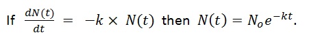
1. The size of a radioactive sample is can be expressed as a function of time:

     N(t)=N_oe^-kt

2. The graph of this function looks like this:

Note that at time = 0, the value is N_o and then the value decays asymptotically toward zero.

3. Graphs like this show up in many other contexts.  For example, this looks a lot like the graph of current vs. time for a charging capacitor.  It also looks like the graph of acceleration vs. time for an object in free-fall with air resistance.  And there are a number of graphs associated with motors and generators that also have this shape.

4. When a quantity decays exponentially, in equal time intervals it will decrease by the same factor.  Most notably, the time it takes to decrease by 50% is called the “half-life”.  There is a useful formula relating the half-life to the decay constant:

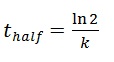
Do NOT just memorize this – derive it for yourself.  If you need help getting started, you can begin by letting N(t)= ½ N_o.

*** To see that this claim about half-life is true, you can play with Part 1 of the desmos activity here:  https://www.desmos.com/calculator/ooewvdzrmq

However, all of this assumes that we already know that the function is N(t)=N_oe^-kt . But how do we know that?  When you see exponential decay, you should suspect that somewhere behind the scenes lurks something called a differential equation.  And that brings us (finally) to the topic of this post.

WHAT IS A DIFFERENTIAL EQUATION?

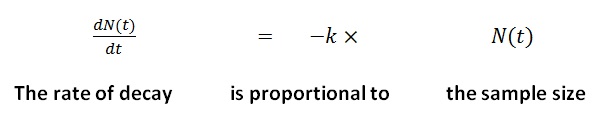
“The rate at which a given radioactive sample decays is proportional to the size of the sample.”

I hope that sentence makes sense to you, intuitively.  It is saying that when there are more nuclei available to decay, the decay rate is faster.  As the sample shrinks in size, there are fewer available nuclei and so the rate slows down.

*** This claim can be investigated further in Part 2 of that same Desmos activity: https://www.desmos.com/calculator/ooewvdzrmq  Really, go do this now!  I’ll wait here…

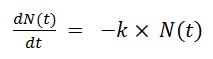
OK, so the rate is proportional to the current value.

But that sentence can be re-written using mathematical symbols:

The resulting equation relates a function, N(t), to one or more of its derivatives.  In this case, the highest order derivative is the first derivative so this is called a “first order differential equation”.  We are going to encounter a number of these in AP Physics and also a handful of second order differential equations as well.  You will learn how to solve some of these in math class this year.  If you continue in math and science, you may spend a number of semesters learning more about this topic.  For now, I am going to show you a method that will be sufficient for our specific needs.

 WHAT IS A SOLUTION?

When you solve an algebraic equation, you find a number that you can use in place of the variable, thus obtaining a true statement.  For example, x= 3 is a solution to the equation 2x + 4 = 10 because when you replace x with 3 in that equation, you get a true result.  And even if you didn’t learn the step-by-step method of solving that equation, you could still verify that x=3 works.  It wouldn’t matter if the solution came to you in a dream!  Once you verified it, you’d know you were right.

Now we have a different kind of equation:

We are not looking for a number.  We are looking for a function, one that will make a true statement when we use it to replace N(t) in that differential equation.  Here is how we are going to do this:

(Don’t worry if this doesn’t “click” at first.  We will walk through this several times.)

1. Based on our intuition, draw a graph of what the function N(t) will look like.

2. Use our extensive knowledge of pre-calculus to guess a general form of a function that has that a graph shaped like the one we just drew.

3. Take the derivative of our guess (and second derivative if needed).

4. Substitute back into the equation we are trying to solve to see if we get a true statement.

If we have guessed correctly (as we often will), we will actually pick up some bonus information.  Follow along with me and see what I mean.  We’ll start from the beginning.

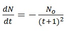
We are seeking a function N(t) that will satisfy this differential equation:

1. Our intuition about radioactive decay suggests that when we find the solution, its graph, as we already noted, will look like this:

2. There are a number of functions that have that shape.  For example, it could be that:

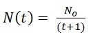
It’s not a terrible guess. It has the right value at t=0 and it approaches zero asymptotically.  I don’t remember seeing that function used to model decay before and it would be all wrong for t approaching -1, but let’s try it anyway.

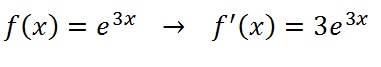
3. Taking the derivative, we get…

4. Now, substituting the function and its derivative back into the original differential equation, we get:

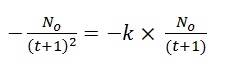
Hmm…can this be true?  For a given value of k, it is true at some particular time. But we want a solution that is ALWAYS true.  There is nothing we can do to fix this one.  It turns out that our initial guess, though not terrible, was wrong.  OK, new guess.  Let’s try an exponential function.  Our memories from pre-calc  give us high hopes for this one:

In this case, we would have the derivative:

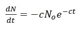
(because the derivative of “e to the something” is “e to the something” and then there is that chain rule multiplier.)

But what happens when we substitute these expressions back into the original differential equation?

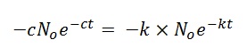
Can this be true? Why yes, but only if c = k.  In other words, we have just learned that we had correctly guessed the general form of the solution but it can’t be just any old exponentially decaying function.  The decay constant in the function has to match the constant of proportionality in the original differential equation.  So with that adjustment, we have our solution:

This kind of thing happens a lot when we use this technique.  At the end of the process, when you ask, “can this equation be true?” you get as the answer: “yes, but only if…” followed by some new information that tells you the required value of some constant.

Closing remarks

Please do not worry if you have found this post to be challenging.  In the next practice set, I will give you a couple of additional examples and walk you through this process step-by-step.  And we will also do a couple together in class.  But review this a few times and you may realize that it is just another way to make use of derivatives and we still have not used any rules beyond the ones I showed you in the earlier posts.  But that does not mean that this was easy!

A Very Useful Thing About Slope Formulas

As you have worked through the previous posts and exercises, I hope you have noticed something special about places on a graph where the derivative is zero.  These places have horizontal tangent lines.  And in their own neighborhoods, they are often a local maximum or local minimum.  This piece of information is very helpful when you are trying to solve an “optimization” problem.

For example…

Suppose you are firing a projectile on a horizontal surface at a fixed launch speed, v.  And let’s also suppose that air friction is negligible.  What angle will maximize the range (horizontal distance) of the projectile?

You may remember the answer from your first year of physics.  It is intuitive and there was a way to get the answer without calculus.  But we can still use this example to illustrate the calculus method.

(Graphic from http://outreach.phas.ubc.ca/phys420/p420_00/darren/web/range/range.html where you can also see a review of the projectile physics)

STEP 1: Express the quantity to be optimized as a function of a single variable.

In this case, a review of that website or last year’s notes will remind you that the distance varies with the launch angle by the rule:

In brief, we resolved the launch velocity into components, used the vertical component to determine time in air and then multiplied that time by the horizontal component of the velocity.  But now that we have this expression, for our current purposes it would be helpful to make use of the double angle identity for the sine function.  We can write:

Don’t worry if you would not have remembered how to do all that without notes.  The point is to learn what we can do with this expression now that we have it.

STEP 2: Find the derivative

This is one we know how to do:  we know the derivative of sine functions and we know the special case of the chain rule.

STEP 3: What is the domain of interest to us?

When a math book asks for the domain of a function, they usually mean the largest, most inclusive domain possible.  For a sine function, that would be all real numbers.  But that is not what we are after here.  We need to think about the portion of the domain that is relevant.  To fire this cannonball as far as we can, clearly we will choose an angle between 0 and π/2 radians.

STEP 4: Where in that domain is the derivative equal to zero?

In this case…

(OK, call it 45 degrees if you prefer.)

 STEP 5: (Your math teacher may not like this) Convince ourselves that we are done.

In math class, once you have found where the derivative is zero (or undefined), you are not nearly done.  You have to investigate each of these “critical points” to see what kind of extreme it is and to justify your conclusion with such things as sign charts and 2^nd derivative tests.  But in physics class, you are going to get away a little easier because of the following claim:

If a “smooth” function has only one critical point on some interval and the value of the function is higher at that critical point than at either of the endpoints, then that value is the “absolute maximum” value.

So in the example at hand, we know the cannonball’s range is zero when the angle is zero, and its zero when the angle is 90 degrees (as the ball goes straight up and down).  But it is NOT zero when the launch angle is 45 degrees.  But the tangent line is horizontal at 45 degrees.  So that’s the “best” angle.

You still have to learn to do things the math-class way.  There are lots of functions with multiple critical points.  And there are functions that have horizontal tangent lines at places that turn out not to maxima or minima.  So you do have to know how to investigate further.

But the problems you will see in AP Physics don’t turn out that way.  Most often, there will be only one critical point and it will be the one we were looking for.  Here is another example I have always liked.

Suppose you have a large cylindrical tank full of water, open at the top.  You are going to punch a hole in the tank somewhere along its side and you want the resulting jet of water to land as far from the tank as possible.  Where should you make the hole?  And where will that initial jet of water land?

Let’s say you make the hole y units from the ground and the initial jet lands x units from the tank.

STEP 1: Determine x as a function of y

First we need the “speed of efflux” which you can think of as the horizontal launch velocity of the water coming out of the hole.  There is a neat result from fluid dynamics that shows that the water leaves the tank at the same speed as if it had free-fallen from the top of the tank.  It’s called Torricielli’s Law.

You can see more about this calculation here:

http://en.wikipedia.org/wiki/Torricelli’s_law  (where I also got the graphic above)

Now, we just find the time in air and multiply by that launch speed.

For time in air, we can use the fact that

and solve for time to get:

So for the distance as a function of the height of the hole we get:

STEP 2: Find the derivative

Well, it seems we need the more advanced version of the chain rule. But there is a trick to make things easier.  The distance x will be at its maximum when the term inside the square root is at its maximum.  So let’s ignore the square root and just maximize the innards.

STEP 3: Domain of interest?  We can’t make a hole below the ground or above the height of the cylinder so we only have to consider y values between 0 and h.

STEP 4: Set the derivative equal to zero

We need a hole in the middle!

 STEP 5:  Convince ourselves that we are done

There was only one critical point.  And the endpoints both lead to a distance of zero.  So the hole at y=h/2 is the one that gives us the farthest landing point.

And what is that landing point? Substitute y=h/2 into our original function, which was:

I will leave the substitution and clean-up to you.  I will say that it cleans up quite nicely and has a memorable result.  The first of my students to post the correct result in a comment wins some silly thing or other.

Quick Recap and Closing Remarks

In AP Physics, when you want to find the maximum or minimum possible value of some quantity, most of the time it will just be a matter of taking a derivative, then setting it equal to zero and then waving your hands around to convince us that you are done.

The hardest part of the process is not going to be the calculus.  It’s going to be setting up the variables and finding the expression for the quantity you hope to optimize.  That’s why you had all those homework problems back in pre-calc that said “Express this thing in terms of that thing”.

I guess I should mention that if you are having trouble either finding the derivative or solving after you set it equal to zero, you may find your TI82 to be of some use.  But honestly, sometimes it feels like the calculator only gives intelligible answers to people who already know what the solution looks like.

(and some loose ends)

Before we get to the practice questions…

1.  I want to introduce anther notation for derivatives.

Suppose we are working with a function y=f(x)

Instead of writing the derivative as y’ we often write:

The expression is telling you to find the derivative of the function f with respect to the variable x.  For now, this seems like a more cumbersome notation but there will be times when you appreciate its clarity.  It leaves no doubt about what variable you are working with.  This will be critical when you are working with functions of more than one variable.

2. And yet another notation for derivatives, this time a lazier one…

In many instances, the functions we are considering will be functions of time, t.  When we want to indicate that we are taking the derivative with respect to time, we just write a dot over the variable.  So for example, let x(t) be the position of an object as a function of time.  In that case, the velocity would be:

Typically, if we are being this terse, we may as well be briefer and write:

Here we are figuring that by using the dot notation, we are implicitly saying that these are both functions of time.

And then we can say things like:

This is just a concise short-hand for “acceleration is the derivative of velocity with respect to time and the second derivative of position with respect to time.”

OK, this brings us to the practice set.  I have posted it here as a pdf.  Note to my Holmdel students:  I have also emailed it to your school account.  So if you did not get it, you should email me to ask to be added to the mailing list.  If you have any questions, post them here as comments (Holmdel student or not).

Practice Set #1 AP Physics Math Preview

Suppose we want to find a derivative for this function:  h(x) = sin(2x).

The sine function is on our list – we know that the derivative of sin(x) is cos(x).  But we are not dealing with just the sine function.  There’s another function inside the function!  We don’t just have “sine of x” but rather we have “sine of something”, where the “something” is itself a function.

This means that to find this kind of derivative, it is essential that you have a clear understanding of the composition of two functions.  You have to look at  h(x) = sin(2x) and see it as the composition of functions and you have to recognize the building blocks:

g(x) = 2x and f(x) = sin(x)

We are not going to just add them or multiply them.  Instead, we use the output of one of them as the input to the other. So we build:

  h(x) = f(g(x)) = sin(2x)

The g function is the inner function.  It starts off by doubling its input.  Then that output is handed off to the “outer function”,  f  which finds the sine.

And now, it we want to find the derivative, we need to learn…

THE CHAIN RULE (maybe)

 Once again, I have to pause and remind myself of the purpose of these posts. If I show you  “the chain rule”, we can then use it to start finding derivatives of long, challenging “chains” of compositions of multiple functions, such as:

But then I remember two things:

1. This is beyond what we will actually need in the opening months of AP Physics.

2. Your math teacher deserves to have some of the fun as well.

So I am only going to introduce a lesser version of the chain rule, one that is just enough to handle a special case, one that we will actually need in class very early in the year.

THE SIMPLE CHAIN RULE FOR CONSTANT MULTIPLIERS

For example, look at each of these:

In each case, the “outer” function is one from our list of well-known functions.  And the “inner” function is a constant multiplier.

There is an easy rule that handles all of these:

In other words, go ahead and take the derivative using the familiar rule, but then multiply your answer by the constant you see “inside” the original expression.

With this rule we can find all three of the derivatives above:

The derivative of “e to the something” is “e to that something”, and the 3 is a multiplier.

The derivative of “the cosine of something” is “the minus sine of that something” and the 5 is a multiplier.

The derivative of “the sine of something” is “the cosine of something” and the 2 is a multiplier.

 DON’T JUST TAKE MY WORD FOR IT…

Why do we multiply by that same number you see in the inner function?  It turns out that there is an intuitive way to understand this rule.  Once again, we have to look at graphs and their transformations.

In the last post, we saw that compared to the graph of y = f(x), the graph of y = a·f(x) was stretched vertically when a>1, and that the vertical stretch affects the tangent line as well, also increasing its slope by that same factor, a.

But now we consider the graph of y = f(a·x), we see that a>1 leads to a horizontal compression, and that compression affects the tangent line as well.  Slope is rise over run, so reducing the run increases the slope, again by that same factor, a.  That’s why our derivatives all have that multiplier: compressing the graphs horizontally makes the slopes steeper.

For example, here are graphs of f(x) = e^x and f(x) = e^3x.

You can see that the graph is horizontally compressed.

And when you compare the slopes of the tangent lines, you see that the second one is 3 times as steep as the first. [But notice: the first tangent line is at x=.6 and the second one is at x=.2.  Why did I do that?  Post a comment with your answer…]  Until your math teacher unveils the chain rule in its full glory, please let the diagram above serve as a proof of our simpler version. But in the mean time…

Here is an animated version of what I am trying to say:

And if you want to play with the Desmos file, it’s here.

SO WHERE ARE WE NOW?

At this point, we have assembled some basic derivative formulas and some rules about combining them.  This would be a good place to pause and see if you are keeping up.  So in the next post, you will find a set of practice questions.  Once you have mastered them, you will be ready to find out what we do with these slope-finding formulas once we have derived them.

In the last post, we compiled a small collection of derivative formulas, formulas which will enable you to find slopes of tangent lines.  (Why you would want to do such a thing is a discussion that is coming soon.)

You will see all of those functions in various settings as you study AP Physics.  But they don’t always act alone.  You have to be able to work with combinations of those functions in some ways that are intuitive but others that are, well, less intuitive.

1. Adding and Subtracting — Just as you would guess

Suppose f(x) =x³ +x²

and you would like to find the derivative.  You might be thinking:

“Wait — I have a rule for each of those terms, separately.  Can I just add them? ”

In other words, is f'(x) = 3x² + 2x ?   Yes it is.  We could say this more officially:

If h(x) = f(x) + g(x) then h'(x) = f'(x) + g'(x).

But all that means is that if you have functions added together, you can use their separate derivative formulas and then add them.  And it works the same way for subtraction.

2. Multiplying by a Constant — Also as you would guess

Given f(x) = 3sin(x)…yes, it’s true: f'(x) = 3cos(x).  Multiplying the original function by a constant just multiplies its derivative by the same constant.

There is an intuitive way to see why this must be true:

Consider a function, g(x) = a·f(x), where a>0.   How does the graph of g compare to the graph of f? [SAT fun fact!]  It is vertically stretched or vertically compressed, depending on whether a is greater or less than one.  Now, how would that affect the tangent line?  A vertical stretch by a factor, a, will increase the slope of that tangent line by that same factor, a.

Here is an illustration of what I mean:

On the left, you see the graph of f(x) = √x and its tangent line at x = 1.  The slope of that tangent line is .5.

And on the right, you see the graph of f(x) = 3√x and its tangent line, also at x = 1.  The graph has been stretched vertically by a factor of 3.  And sure enough, the tangent line is 3 times as steep, or 1.5.

We’ll call that a “proof” and state the rule officially:  if g(x) = a·f(x) then g'(x) = a·f'(x).

3. Multiplying and Dividing Functions: NOT what you would expect

Well, it’s a bad new/good news kind of thing…

Bad news: you can’t just multiply the derivatives.  In other words, if h(x) = f(x)·g(x), it would be convenient if  h'(x) = f'(x)·g'(x).  But, alas.  Though we don’t know what the rule is, we know enough to see what it isn’t.

All we have to do is let f(x) = x³ and let g(x) = x².  Then h(x) = f(x)·g(x) = x⁵ .

We also already know the derivatives: f'(x) = 3x² and g'(x) = 2x.  When you multiply them, you get. 3x²·2x = 6x³  But we already know that h'(x) = 5x⁴.  So the product of the derivatives did not match the derivative of the products.  That’s the bad news. And a similar argument can be constructed to show that quotients don’t work that way either.

So what’s the good news?

1.  There are rules that handle these situations.  They are called the product rule and the quotient rule.  I am sure that your math teacher will be happy to teach them to you.

2.  This is where I pause and remind myself what these posts are for.  I am trying to get you ready for your year of AP Physics.  We may need the product rule and the quotient rule before the year is over, but we won’t need them right away.  By the time we do need them, you will have seen them in math class.

On the other hand, there is one more way to combine functions that we will need almost immediately.  So in the next post, we are going to look at something called “the chain rule”.

In the last post, we started with f(x) = x³ + 4x and by some mysterious process, we generated a new formula, f’(x) = 3x² + 4. This “derivative” tells us the slope of the original function’s tangent lines. 

As you enter AP Physics, I would like you to be able to find the derivatives of some basic functions.  I will let your math teachers explain where these formulas come from, but I want you to start getting familiar with these now.

Also, It is true that a TI-89 can find these derivative formulas for you.  But the ones I am asking you to learn are so frequently encountered that it would be a waste of time to have to reach for a calculator.  So let’s begin:

1. Constant Functions

Suppose f(x) = c, where c is a constant.  The graph of f will be a horizontal line.  The slope everywhere on that line is zero.  So our first rule is an easy one:

If f(x) = c then f'(x) = 0

2. Linear Functions

Suppose f(x) = kx, where k is a constant.  This graph will be a line passing through the origin with a slope, k.  So this rule is also straight-forward:

If f(x) = kx then f'(x) = k

3. The Power Rule

Some examples: 

f(x) = x²         →       f’(x) = 2x

f(x) = x³         →        f’(x) = 3x²

f(x) = x⁴         →        f’(x) = 4x³

 4. Power Rule, Special Cases

The power rule works for negative powers and for fractional powers.  So you can use it to figure out the next two examples.  But I think these two are worth memorizing so that you don’t have to stop to re-derive them…

5. Two Trig Functions

Your math teacher will teach you the derivatives of the functions for all six trigonometric ratios (and their inverse functions!) but for now, I’m just asking you to learn these two:

 f(x) = sin(x)   →        f’(x) = cos(x)

f(x) = cos(x)   →        f’(x) = -sin(x)

If you would like to be convinced that the derivative of the sine function is the cosine function, play the video.

Watch the tangent line surf along the sine wave (blue).  Its slope changes in a pattern that matches the values of the cosine function (pink).

 6. One more interesting function

There are many, many applications of exponential growth and decay in physics.  Exponential functions are in the form:

where b is the base and x is the exponent.

Here is the graph for the case when b = 2:

As long as the base is greater than one, exponential functions will all have this same characteristic shape.

There is, however, one special value for the base: the Euler number, e = 2.7182…

I sometimes think of e as π’s neglected cousin.  They are both “transcendental” numbers, but I don’t know of any middle school that holds competitions for memorizing the digits of e. That may be because π is easier to explain:  it’s the ratio of a circle’s circumference to its diameter. 

But what is e?  That’s a longer story (maybe for a future post — though there are entire books devoted to this subject).  For now, I will tell you an interesting and important fact about e.  The exponential function that has e as its base has a special property:

At every point along the graph of the function f(x) = e^x, the slope of the tangent line at that point is equal to the value of the function at that same point.

Stop the movie at any point.  Compare the value of the function to the slope of the tangent line until you can say “Aha!”

This gives us one more derivative rule:

Enough to Build on…

The basic rules you have seen in this post will get us through most of AP Physics.  Now we have to learn how to apply these rules to combinations of functions.  That’s coming next.  For now, I’ll close by re-listing the rules.  Memorize them.  Print them out and put them in your notebook.  Know them like you know your times-tables.

By the end of this post, you will know what a derivative is.  You won’t know how to find one yet, but you will know what you have if you are given one! 

Let’s say that we were given a function such as f(x) = x³ -4x.

We know it isn’t a linear function so when we graph it, we are not surprised to see the curves.  And if you can imagine a tangent line “surfing” along the curve, the slope of the tangent line would clearly be changing as you went along.  Here’s what I mean:

If you wanted to know the slope at a given point, you could estimate it by drawing the tangent line and then finding the slope of that tangent line (as we have seen in the last post).

But there is an alternative to that method that is useful and quick.  When you have the rule for a function, there is a way to derive a formula for a new function that will give you the slope of the original function’s tangent line at any x-value you choose.  Since it is derived from the original function, this new function is called “the derivative” of the original function.

For example, if the original function is:

f(x) = x³ – 4x

The derivative is written:

f’(x) = 3x² – 4

The symbol f’(x) is pronounced “f-prime of x” and it is the most commonly used symbol to represent the derivative of the function f.

TWO THINGS YOU SHOULD NOT WORRY ABOUT (YET)

1. How did we get from the function f(x) = x³ – 4x to its derivative f’(x) = 3x² – 4?

I will show you how to “take a derivative” in the next post.  Once you learn a handful of rules, the process is not difficult.  It’s easier than factoring.  It’s easier than long division.

2.  Why would anyone want a slope-finding formula ?

Once you know how to take derivatives, I can show you a variety of ways that they are useful.  In fact, you’ll even get to use them forward and backwards! (That was supposed to be some fore-shadowing…)

For now, my goal is simpler.  I just want to be sure that we understand what it is that the derivative formula tells us.  And once again…it’s better with diagrams.

I made the graphs and videos in this post using a web-based applet written by Paul Seeburger, a professor of mathematics at Monroe Community College in New York.  You can find the applet at:

http://web.monroecc.edu/manila/webfiles/pseeburger/JavaCode/DerivativeDemo2.htm

The blue line is the original function, f(x) = x³ – 4x. 

The purple line is the derivative, f’(x) = 3x² – 4.

The red line is the tangent line.  You can calculate the slope of that tangent using rise over run if you want to, but you don’t have to.  The applet does the calculation for you – look in the pink box.

Now let’s pick a point on the graph and examine all of the lines on this diagram.

At x = -2, f(-2) = (-2)³ – 4×(-2) = -8 + 8 = 0.  This means that (-2,0) is a point on the graph of f.

At that same point, the tangent line has a slope of 8 (as you can see in the pink box).

If we plug x = -2 into the derivative formula, we get f’(-2) = 3(-2)² – 4 = 12 – 4 = 8.  And then, when you look at the graph of the derivative (in purple), you see that (2,8) is a point on that graph.  So the derivative formula tells us the slope – at least at that one point.  But does it always work?

Well, let’s look at another point:  x = -1.

(If you are playing along at home, you can enter any x-value you want into the box on the lower left hand side of the applet where it says “Trace x =”)

At x = -1, f(x) = (-1)³ – 4(-1) = 3.  So (-1, 3) is a point on the graph.

Then, f’(x) = 3(-1)² – 4 = -1.  So we expect the slope of the tangent line to be -1, and it is. You can see that (-1,-1) is a point on the graph of the derivative (again, the purple one). So once again, the derivative formula has given the slope of the tangent line.

Here’s one more point that is worth noticing:

Look at the value of the derivative.  And then look at the shape of the graph.  Where the derivative is zero, the graph has a horizontal tangent.  That little fact turns out to be a big part of one of the reasons why we care about derivatives. They help us to find places where the graph has a maximum or (as in this case) a minimum.  We’ll be hearing more about that later.

So we have confirmed, at least for the points we checked, that for this particular function, the derivative formula does in fact give values that match the slopes of the original function’s tangent lines.   If you want to, you can check many more points:

As you saw in the video above, Professor Seeburger’s applet lets you trace along the graph.  As you do, the tangent line surfs along the curve and the applet keeps track of all of the values.  Here is that video again, this time with the derivative function and the values all visible:

So if you are skeptical, run the video and then pause it wherever you want.  You’ll see that the slope of the tangent line always matches the value given by the derivative.  Derivatives really are slope-finding formulas.

When we examine the graph of your accelerating hair growth, it’s easy to show that the growth rate is increasing.  We can examine average growth rates for successive time intervals.

For example, we could choose to look at 10-week intervals, calculating rise over run for each interval.  You should check for yourself to see that the average growth rate increased from just under 0.5 inches/week over the first 10-week interval to nearly triple that rate over the fifth 10-week interval.

Those are still just average rates.   But what if you wanted to know how fast your hair was growing right NOW!? Not over a finite interval but at a specific moment.   There is a way to answer that question too.  But you may have philosophical or mathematical objections.  “If no time passes, how can ANYTHING have a rate of change?” 

The way we answer this kind of question is by making use of the idea of a limit.  Essentially, to find the slope at a given point, we start by finding the slope between two different points: the point we were asked about and another point a little later. But then we move that second point closer to the first one.  How close?  Reeeeeeeally close but not all the way there.  And as it gets closer, we look to see if there is a value that the slope approaches.  If so, we use that value as the instantaneous rate of change.

 There are many websites that explore this concept in greater depth.  And they have some nice animations.  Here are a few:

http://clas.sa.ucsb.edu/staff/lee/Secant,%20Tangent,%20and%20Derivatives.htm

http://www.math.umn.edu/~garrett/qy/Secant.html

http://www.slu.edu/classes/maymk/Applets/SecantTangent.html

Here is an animation taken from the first website listed above:

 UPDATE:  Now that I have discovered Paul Seeburger’s applet, here is a nicer look at that same idea:

I will leave most of the details for your math teachers to explain.  But I will point out that this is exactly why they want you to learn about limits.  Limits are the mathematical way to say “reeeeally close but not all the way there”.  It’s reasonable to say that limits were invented as a way of dealing with precisely this question: how do we find the slope of a line at a given point?

 As your physics teacher, I want you to know two ways to deal with this question. 

1. WITHOUT CALCULUS

Here is a graphical method that will give us an approximate answer:

(This is the method I use with my 11^th graders.)

Use a ruler to draw a tangent line.  The slope of that tangent line is also the instantaneous rate of change.

So let’s say you wanted to how fast your hair was growing at the end of week #20.  (Note carefully: we are not looking for the average rate over the first 20 weeks.  We are looking for the instantaneous rate exactly at t = 20 weeks!    It’s a different question.)

After you draw the tangent line, you choose any two points on that line and use them to calculate rise over run.  So, using the values we get from the graph above, we calculate that the slope of the tangent line is (15 inches)/(20 weeks) = .75 inches/week. So now we know:

At week #20, the instantaneous velocity of hair growth was .75 inches/week.

 2. WITH CALCULUS

The point of the entire discussion up until this point has really been to remind you about the idea of slope as a rate of change and to introduce (or re-introduce) what we mean by instantaneous rate of change.  But I don’t expect that we will be drawing many tangent lines by hand during AP Physics.  When we need to know the slope of a graph, there are formulas for that kind of thing.  We’ll start looking at those formulas in the next post.

In my last post, I reported on the results of your hair-growing experiment. 

Now suppose that at the end of the year, you go back and analyze your year of hair growth.  You can see from the graph that your hair grew steadily at a rate of 0.3 inches per week.  That was the slope of the graph no matter what time interval you chose to examine.  So we concluded that the rate was constant. 

If we feel like it, instead of graphing hair length, we could graph the graph the growth rate instead. 

This graph is not that exciting.  Since your hair grew at the same rate week after week, this graph is a horizontal line.  But it is important to understand that we are still talking about the same experiment.  The first graph showed hair length.  That graph slopes uphill at a constant rate.  This new graph shows growth rate – it is the slope of the previous graph.  And since that graph had a constant slope, this new graph is horizontal.

 Now let’s suppose that you were not satisfied with the year’s hair growth.  So you search the internet for hair growth accelerators.  (I’m sure people actually do this.)  And let’s also pretend that you find one that really works as advertised.  It promises that if you use it every day, you will experience steadily increasing hair- growth-rates.  In fact, they promise:

Guaranteed Acceleration = .023 inches/week²

Exactly what does this mean? If you are new to physics, it is possible that you don’t know how to interpret this guarantee. I mean, what is a “week squared” anyway?  

Still, you decide to try it.  In the interest of science, you shave off your hair on New Year’s Day and begin the experiment.  Here are your results:

Now that’s some seriously long hair!  In one year, your hair has grown nearly four feet!  And when we look at the graph of growth rate, it is now a little more interesting:

Your rate of hair growth certainly increased.  It was 0.3 inches per week at the beginning of the year.  And by the end of the year, the rate had increased to 1.5 inches per week, increasing by 1.2 inches per week over the course of the year.  But the increase did not happen all at once. The growth rate increased steadily.

By how much did the growth rate increase each week?

We can answer this question two different ways.

1. Since we know that the rate increase for the entire year was 1.2 inches per week, we can divide to find the weekly increase:

1.2 ÷ 52 ≈ .023 inches per week per week

Let’s make sure to understand what we just figured out.  Each week, the growth rate increases by .023 inches per week.  At the beginning of the year, the rate was .3 inches per week.  After 1 week, it will have increased to .3 + .023 = .323 inches per week.  After 2 weeks, it will increase and additional .023 inches per week to .3 + .023 +.023 = .346 inches per week.  In other words:

Hair Growth Acceleration = .023 (inches/week)/week

When we are being lazy, we write:  .023 inches/week²

2. We can also find the growth rate by evaluating the slope of the graph of growth rate.  Just like hair “velocity” is the slope of the graph of hair length vs. time, hair acceleration is the slope of the velocity graph.  And since that graph is linear, we can pick any two points to calculate the rise over run.

Using the points I have chosen, we get a rise of .6 inches per week over a run of 26 weeks which comes out to a slope of .6 ÷ 26 ≈ .023 (inches/week)/week, just as we expected.

But to even draw a graph like this, we must somehow believe that at any given moment in time, your hair is growing at some particular rate.  So now let’s look back at the graph of hair length vs. time:

You can see that this graph is NOT linear.  As time passes, the slope gets steeper because your hair growth is accelerating.  Every instant, the rate is changing.   Again, we seem to be talking about instantaneous growth rates.  That’s our next topic.

The next bunch of posts are intended for my incoming AP-C Physics students.   The course is a calculus-based version of 1^st-year college level physics.  Some of my students will be starting to study calculus just as they are starting this course.  These posts are designed to give them enough of an introduction to stay above water.  So here we go…

 Slope is a rate of change.

Many of the quantities you have already encountered in your study of physics are rates of change of other quantities. For example:

Velocity is the rate of change of position with respect to time.

Acceleration is the rate of change of velocity with respect to time.

Force is the rate of change of momentum with respect to time.

Current is the rate of change of electric charge with respect to time.

Induced Voltage is the rate of change of magnetic flux with respect to time.

And there were many times when you found the rate of change by graphing the quantity vs. time and then evaluating the slope of the resulting line.  Let’s look at a non-physics example.

For one year, you let your hair grow, measuring the length at the end of every week.  You graph the results of your experiment below, along with the line of best fit.

There are some questions that we can answer by reading the information directly from this graph.  For example…

1. How long was your hair after week 10?

2. When did your hair reach a length of 15 inches?

3. How much longer did you hair grow between the end of week 20 and the end of week 30?

(Post a comment if you have answers or questions about any of these.)

Then there are questions that you answer by finding the slope.

4. What was the average rate of hair growth over the first 5 weeks?

5. What was the average rate of hair growth between week 10 and week 20?

6. What was the average rate of hair growth for the entire year?

7. At what rate was your hair growing at the end of week 30?

Questions 4, 5 and 6 are all answered the same way: you find the rise over run to determine the rate of change.  This should remind you of your first weeks in physics class, studying kinematics.  We could even call this slope  the “hair velocity” if we like.  

And in fact, you should get the same answer to all three questions.  The graph is linear.  You will find the same slope no matter what two points you pick.  We can say that your hair is growing at constant velocity.

Question 7 is different from the others in a subtle but important way.  It asks you to find the growth rate at a specific time – and not over a time interval!  It is asking for an instantaneous rate of change, not an average.  Fortunately, this time, it’s still an easy question.  Since we have seen that the growth is at a constant rate, it is reasonable to assume that the rate at any particular instant is the same as the average rate for the entire period (or in fact, any period you pick!  It doesn’t matter – the rate is constant.)

But while that gives us an answer, it also lets us side-step some important questions:

1.  How would we find the rate of change at a given time if your hair growth rate wasn’t constant?

2.  What do we even mean by the rate AT a given time?  Don’t you need to compare TWO times in order to find a rate of change?

We’ll consider these in the nest post when you experiment with some hair-growth-acceleration tonic you found on line.